Foundation of Reinforcement learning(I)

The category of decision making problem

dimension	single step	multi step
one person	optimization problem	RL, to the best situation
multi person	static game	dynamic game, MARL.etc

Dynamic programming

Dynamic program is used to solve the Sequential decision making problem, feature of this problem is that it’s decision making process is sequential, and the decision at one step will affect the next step, and the reward is received at the end of decision making process, not at each step.

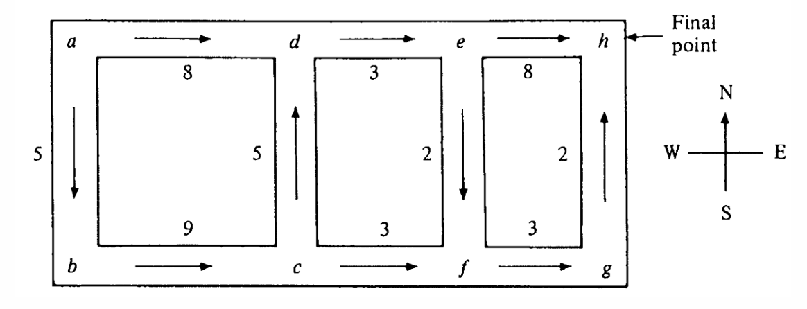
For an example, given a maze like problem below, the agent need to find a way from Position A to Position B, and the time of each way is different. Agent need to find the way with the least time. A simple way to solve this is to list all the possible paths, but if there is a circle, if the map is large, this will be unfeasible.

A better way to solve this is Backward induction, we start from the end point, and for evey point we calculate the time to reach the end point, then we regart the selected point as the new end point, and repeat this process until we reach the start point. This is a dynamic programming method, and it can solve the problem in polynomial time. But due to we need find a backward path, this method is only suitable for DAG, if there is a circle, this method will fail.

The example is just a introduction, we can summarize the features of dynamic programming as follows:

• it start from the end, and caculate the best action for each state.
• it traverse all the states, and for each state, it calculate the best action, and the value of this state.
• it need to define the state, path(state transition), time(online reward)

So it lead to the Principle of Optimality:

An optimal policy has the property that whatever the initial state and initial decision are, the remaining decisions must constitute an optimal policy with regard to the state resulting from the first decision.

Markov Decision Process

Stochastic Process

A stochastic process is a collection of random variables, which can be used to describe the evolution of a system over time. It’s mathematical definition is as follows:$$P(X_{t+1}|X_t,X_{t-1},\dots ,X_0)$$
This means that the probability of the next state $X_{t+1}$ depends on the current state $X_t$ and all the previous states $X_{t-1},\dots ,X_0$.

Markov Process

Compared to stochastic process, Markov process has a stronger assumption, which is “the future is independent of the past given the present”. Mathematically, it’s definition is as follows:$$P(X_{t+1}|X_t,X_{t-1},\dots ,X_0)=P(X_{t+1}|X_t)$$
This means that the probability of the next state $X_{t+1}$ only depends on the current state $X_t$, and is independent of all the previous states $X_{t-1},\dots ,X_0$.

Trying to understand it’s property is that the current state contains all the information about the past, so we can make decision based on the current state without worrying about the past.

Markov Decision Process

Markov Decision Process (MDP) provides a mathematical framework for modeling decision making in situations where the outcome is partly random, partly under the control of a decision maker. An MDP is defined by the following components:

• State space (S): A set of all possible states in the environment.
• Action space (A): A set of all possible actions that the agent can take
• Transition function (P): A function that defines the probability of transitioning from one state to another given a specific action. It is denoted as $P(s’|s,a)$, which represents the probability of transitioning to state $s’$ from state $s$ after taking action $a$.
• Reward function (R): A function that defines the reward received after transitioning from one state to another given a specific action. It is denoted as $R(s,a)$, which represents the reward received after taking action $a$ in state $s$. Sometimes only relates to the State.
• Discount factor (γ): A factor that determines the importance of future rewards. It is a value between 0 and 1, where a value closer to 0 makes the agent prioritize immediate rewards, while a value closer to 1 makes the agent consider future rewards more heavily.

The dynamic feature of MDP

The whole process of MDP is dynamic as follows:

1. The agent observes the current state $s_t$.
2. The agent selects an action $a_t$ based on its policy $\pi (a|s)$, which is a mapping from states to actions.
3. The agent gets a reward $R(s_t,a_t)$.
4. The MDP transitions to a new state $s_{t+1}$ according to the transition function $P(s_{t+1}|s_t,a_t)$.

The total reward that the agent receives over time is often defined as the discounted sum of rewards:$$G_t=R(s_t,a_t)+\gamma R(s_{t+1},a_{t+1})+{\gamma }^{2}R(s_{t+2},a_{t+2})+\dots =\sum _{k=0}^{\infty }{\gamma }^{k}R(s_{t+k},a_{t+k})$$

Markov Policy

In the context of MDP, a policy is a function that depends on the history:$$h_t=(s_0,a_0,s_1,a_1,\dots ,s_{t-1},a_{t-1},s_t)\pi (a_t|h_t)=P(a_t|h_t)$$

But a Markov policy is a special type of policy that only depends on the current state:$$\pi (a_t|s_t)=P(a_t|s_t)$$

---

In the RL setting, we usually assume that the policy is a Markov policy. Why?

The MDP has Markov property, which means the future is independent of the past given the present, so there is no special information in the history that can help us make better decision, so we can just use the current state to make decision.More informally, for any policy relying on the history, we can find a Markov policy that at least performs as well as it does, so we can just focus on Markov policy without loss of generality.proof(the 26th and 27th slides of the lecture)

---

The category of MDP Policy

At the time demension, we can categorize the policy into two types:

• Stationary policy: A policy that does not change over time. It is defined as $\pi (a|s)$, which means the action taken in state $s$ is the same at any time step.
• Non-stationary policy: A policy that can change over time. It is defined as ${\pi }_t(a|s)$, which means the action taken in state $s$ can be different at different time steps.

At the probability distribution demension, we can categorize the policy into two types:

• Deterministic policy: A policy that always selects the same action for a given state. It is defined as $\pi (s)=a$, which means the action taken in state $s$ is always $a$.
• Stochastic policy: A policy that selects actions according to a probability distribution. It is defined as $\pi (a|s)=P(a|s)$, which means the action taken in state $s$ is selected according to the probability

---

In the RL setting, we usually assume that the policy is a stationary policy. Why?
Typically, we consider the infinite horizon setting. There is also a proof that for any non-stationary policy, we can find a stationary policy that at least performs as well as it does, so we can just focus on stationary policy without loss of generality. proof(the 29th and 32th slides of the lecture)

---

The best policy for MDP

There is a theorem:

In a situation that the discount factor $\gamma <1$, while the state and action space are finite and the horizon is infinite, there exists a deterministic
and stationary policy ${\pi }^{\ast }$ that is optimal, which means for any policy $\pi$, we have $V^{{\pi }^{\ast }}(s)\ge V^{\pi }(s)$.

Proof: Puterman, Martin L. Markov decision processes: discrete stochastic dynamic programming. John Wiley & Sons, 2014.

The goal of MDP

Our goal is to choose the action to maximize the expected reward, which is defined as follows:$$\text{E}[R(s_0,a_0)+\gamma R(s_1,a_1)+{\gamma }^{2}R(s_2,a_2)+\dots ]=\text{E}[\sum _{t=0}^{\infty }{\gamma }^{t}R(s_t,a_t)]$$

So we can define the value function for a policy $\pi$ as follows:$$V^{\pi }(s)=\text{E}[\sum _{t=0}^{\infty }{\gamma }^{t}R(s_t,a_t)|s_0=s]$$
This means the expected reward that the agent can get starting from state $s$ and following policy $\pi$.

Occupancy Measure

In MDP context, the occupancy measure is a way to represent the discounted state-action expectation under a policy $\pi$, also known as state-action visitation distribution. It is defined as follows:$${\rho }^{\pi }(s,a)=\underset{a\sim \pi (s),,s’\sim p(s,a)}{\mathbb{E}}\left[\sum _{t=0}^{\infty }{\gamma }^t\mathbb{I}(s_t=s,a_t=a)\right]$$

while the $s\sim p(s,a)$ means the state transition, which is defined as follows:$$s_{t+1}\sim p(s_t,a_t)$$

On the other hand, the state occupancy measure is defined as follows:$${\rho }^{\pi }(s)=\underset{a\sim \pi (s),,s’\sim p(s,a)}{\mathbb{E}}\left[\sum _{t=0}^{\infty }{\gamma }^t\mathbb{I}(s_t=s)\right]$$

How to compute the occupancy measure?

State occupancy measure

We assume that the initial state distribution is $\mu (s)$, then we can compute the state occupancy measure as follows:$${\rho }^{\pi }(s’)=\mu (s’)+\gamma \sum _s{p}^{\pi }(s’|s){\rho }^{\pi }(s)$$

then we can solve the fomula:$${\rho }^{\pi }={\left(I-\gamma (P_{SS’}^{\pi }{)}^T\right)}^{-1}\mu$$

State-action occupancy measure

We can compute the state-action occupancy measure as follows:$${\rho }^{\pi }(s,a)=\mu (s’)\pi (a’|s’)+\gamma \sum _s{p}^{\pi }(s’|s){\rho }^{\pi }(s,a)$$

Pay attention that the whole process is flow conservation. Because the state-action occupancy measure is the expected discounted number of times that the agent takes action $a$ in state $s$, so the total flow into state $s$ must equal the total flow out of state $s$. This is why we have the flow conservation constraint in the computation of occupancy measure.

Some Properties of Occupancy Measure

Obviously, from the definition of the measures:

• ${\rho }^{\pi }(s)={\sum }_a{\rho }^{\pi }(s,a)$
• ${\rho }^{\pi }(s,a)=\pi (a|s){\rho }^{\pi }(s)$

We have two important theorems about the occupancy measure:

• Theorem 1: For two policies $\pi$ and $\pi ’$ interacting with the same dynamic environment, if ${\rho }^{\pi }={\rho }^{\pi ’}$, then ${\pi }_1={\pi }_2$.
• Theorem 2: Given a Occupancy measure $\rho$, the only policy that can generate this occupancy measure is ${\pi }_{\rho }(s,a)=\frac{\rho (s,a)}{{\sum }_a\rho (s,a)}$.

Accumulated reward for a policy

As we have defined the occupancy measure, we can compute the accumulated reward for a policy $\pi$ as follows:$$\begin{array}{rl}\mathbb{V}(\pi )& =\underset{a\sim \pi (\cdot |s),s’\sim p(\cdot |s,a)}{\mathbb{E}}\left[R(s_0,a_0)+\gamma R(s_1,a_1)+{\gamma }^{2}R(s_2,a_2)+\dots \right]\\ & =\sum _{s,a}\underset{a\sim \pi (\cdot |s),,s’\sim p(\cdot |s,a)}{\mathbb{E}}\left[R(s,a)\right]{\rho }^{\pi }(s,a)\\ & =\sum _{s,a}R(s,a){\rho }^{\pi }(s,a)\\ & =\underset{{\rho }^{\pi }}{\mathbb{E}}\left[R(s,a)\right]\end{array}$$

Value function and Q function

The value function is used to evaluate a state or a state-action pair, given a policy $\pi$.

The state value function is usually know as value function, which is defined as follows:$$V^{\pi }(s)=\underset{a\sim \pi (\cdot |s),s’\sim p(\cdot |s,a)}{\mathbb{E}}\left[R(s,a)+\gamma V^{\pi }(s’)\right]$$

The state-action value function is usually know as Q function, which is defined as follows:$$Q^{\pi }(s,a)=\underset{a’\sim \pi (\cdot |s’),,s’’\sim p(\cdot |s’,a’)}{\mathbb{E}}\left[R(s,a)+\gamma Q^{\pi }(s’,a’)\right]$$

---

Obviously, we have the relationship between the value function and the Q function:$$V^{\pi }(s)=\sum _a\pi (a|s)Q^{\pi }(s,a)$$
And we can also compute the value function and Q function using the occupancy measure as follows:$$\begin{array}{rl}{V}^{\pi }(s)& =\sum _{a}R(s,a){\rho }^{\pi }(s,a)\\ Q^{\pi }(s,a)& =R(s,a)+\gamma \sum _{s’}p(s’|s,a)V^{\pi }(s’)\end{array}$$

---

Summary

• MDP provides us a simple but powerful mathematical framework to model the sequential decision making problem.

• The five-tuple of MDP is defined as $(S,A,P,R,\gamma )$, which represents the state space, action space, transition function, reward function and discount factor respectively.

• Markov poverty is the key assumption of MDP, which means the future is independent of the past given the present.

• Policy is the function to choose the action, usually is a conditional probability distribution over actions given states, and we usually assume that the policy is a stationary policy.

• Occupancy measure is a way to represent the discounted state-action expectation under a policy, which can be used to compute the accumulated reward for a policy.

• State value function and state-action value function are used to evaluate a state or a state-action pair, given a policy, and they can be computed using the occupancy measure.